The ultimate guide to process factory performance

Factory performance in the process industry (food & beverage, sheet goods, solid & fluids packaging) is different to factory performance in the car industry where most of the continuous improvement methodologies were designed.

In this guide you will learn:

– The building blocks that make up your broader supply chain
– The performance leverage points in your supply chain and where they are located in your process factory
– The difference between a process factory and a car factory
– How a schedule effects factory performance
– The best performance metrics for a process factory
– How to modify Lean, 6 Sigma and Theory of Constraints methodologies for your process factory
– The most important ingredients for process factory performance improvement

Scroll down or download the PDF version of this eguide

Click the link to go directly to the heading

Introduction – The 10 high-powered building blocks that change the way you look at your complex supply chain

Step 1 – Identify the 9 most important operational leverage points in your complex supply chain

Step 2 – Understand the 7 fundamental differences between process factories and car factories

Step 3 – Identify the 7 essentials of your process factory scheduling cycle

Step 4 – Monitor the best top-level performance metric at your process factories

Step 5 – Introduce the 7 most important shop-floor metrics at your process factories

Step 6 – Modify the Lean, 6 sigma and TOC methodologies for your complex process factories

Step 7 – Introduce the 3 essential ingredients of a successful process factory performance improvement strategy

Introduction - The 10 high-powered building blocks that change the way you look at your complex supply chain

Ever wish that there were simple, fundamental building blocks that could be used to represent your supply chain, no matter its complexity?

Hidden in the industrial engineering literature are 10 building blocks that can be used to show the performance of an entire supply chain.

When we think of complex supply chains, we often think of terms such as bullwhip effect, advanced planning & optimisation, sales and operations planning, Lean, Six Sigma, the list goes on.

When all the layers are peeled back however, there exists a basic framework that underpins every supply chain and forms the basis on which we can

link the different parts and functions of a business
link the flow of products, materials and resources to the profitability of a business
identify bottlenecks that are hindering the profitable flow of products

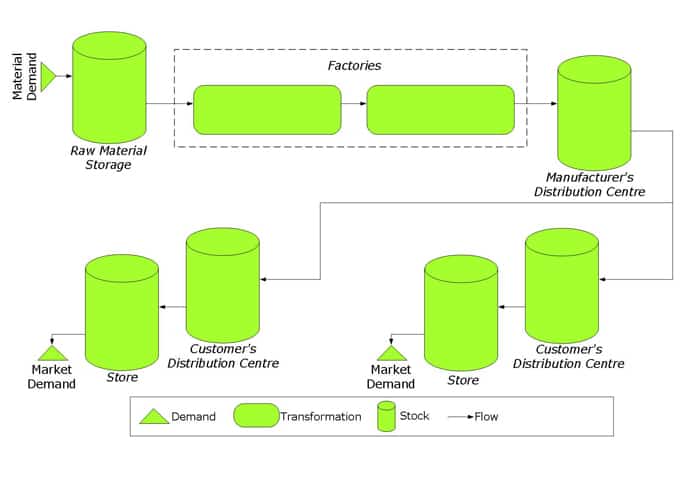
The first 4 of the 10 building blocks are primitive building blocks, fundamental elements that exist in all supply chains.

Building Block #1 - Demand

A measure of customer’s desire and willingness to pay a price for a specific good.

Building Block #2 - Transformation

The act of changing materials, or other resources, into goods in order to meet demand.

Building Block #3 – Stocks

Materials, resources or finished products waiting for transformation or demand.

Building Block # 4 – Flow

Materials, resources or finished products moving to, through or from transformation processes or stocks

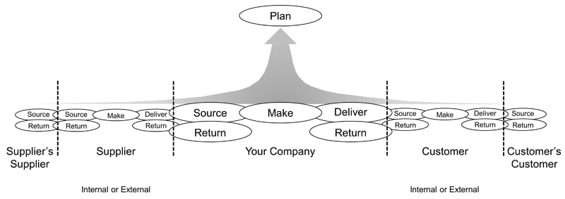
These building blocks can be connected together to represent a supply chain. Here we have a simple retail supply chain.

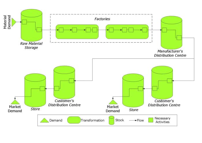
Each transformation process can be split into any number of necessary activities. Also, stock locations such as warehouses involve other necessary activities including a number of unloading, putaway, picking and loading activities.

This brings us to our next building block.

Building Block #5 – Necessary Activities

Necessary activities can be fully manual through to fully automatic activities. These activities can be necessary but non-value adding OR necessary and value adding. In any case they are recognised as necessary activities within the supply chain.

This would be a good and helpful model if demand and transformation behaved in a deterministic way. This model would be helpful if we could perfectly predict when a customer wants product and know that factories and resources could transform product with a reliability of 100%. In this case stocks could be restricted to only those required to fulfil customer sequencing needs.

However, in the real world;

perfection is impossible, or
if perfection where possible it would be impossibly expensive

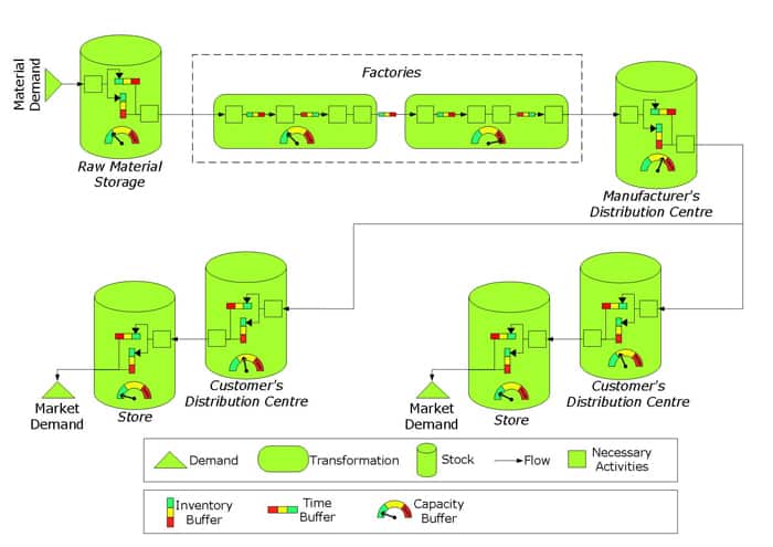
So, to satisfy variable demand using imperfect necessary activities, shock absorbers (or buffers) must be introduced into the system. These behave just like shock absorbers on a car, adjusting to sudden and unanticipated shocks from the road terrain to keep the driver safe.

In this case we are keeping the customer safe from the uncertainties and shocks that occur in our supply chain.

There are ONLY 3 types of buffers that can be inserted into a supply chain.

Building Block #6 – Inventory Buffer

Extra material between 2 transformation processes or between transformation processes and demand.

Building Block #7 – Time Buffer

Early arrival of material or resources before necessary activities, before transformation processes or before demand.

Building Block #8 – Capacity Buffer

Extra potential capacity in necessary activities or transformation processes needed to satisfy irregular or unpredictable demand rates, otherwise known as “sprint capacity”.

There is more information on buffers in the article Buffers! the secret behind exceptional supply chain performance.

Building Block #9 – Rope

“Rope” is a Theory of Constraints term. It represents the gating mechanism used to manage make and distribution signals within a supply chain.

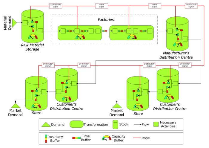
These building blocks can be used to represent a supply chain and its not to hard to think of a way we could animate this conceptual framework. We could use colour coded meters and gauges to represent flow, the depletion of stocks and the flexing of buffers. This would create a compelling show and mesmerise us as we witnessed a complex adaptive system in motion.

The performance of the system could be measured by how frequently different buffers got to dangerous levels. This would be helpful but it would fail to do two things:

identify when we miss supply obligations completely
identify specific bottlenecks that cause supply disruptions

To do this a final piece of the puzzle must be introduced;

Building Block #10 – The Control Point

Control points are placed before and after time buffers or inventory buffers. They measure the frequency with which products, materials or resources were unavailable at crucial points within a supply chain.

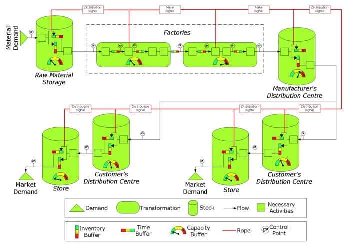
These building blocks can be used to represent any supply chain. Why is this helpful?

These 10 building blocks are the essential elements of Value Stream Maps for the process industry. They provide a means by which planned structural modifications to a supply chain can be represented; communicating the impacts on flow by using a current state map and a future state map. When combined with financial data, showing total-cost-to-serve, this provides a more comprehensive view of supply chain improvement proposals.
The building blocks provide a skeleton on which the flesh of data can be hung. We can choose to introduce data to all the building blocks or we can take a more forensic approach, using data to confirm our perception of how we think the supply chain is operating at a specific point.
Together the building blocks provide a systemic view of the supply chain. For example, while minimising the size of all the buffers is important (i.e. Lean), its important that buffer sizes are only reduced with an understanding of how the changes will impact the rest of the system.

Having introduced the building blocks of supply chains we now turn our attention to identifying the most important operational leverage points in a complex supply chain.

Step 1 - Identify the 9 most important operational leverage points in your complex supply chain

What does your customer value? The harsh reality is that customers often don’t care if your plant is state-of-the-art. They generally don’t care if your warehousing and transportation network is cutting edge.

Usually, what they care about is how quickly products move to and through their supermarket or factory, whether the product is to specification and safe, and whether the product is a good price.

Therefore;

Speed
Quality and Product Safety
Costs (Price)

are often the crucial value-adding factors from a customer’s perspective.

So, what are the key operational leverage points in your complex supply chain that deliver on this value proposition?

There are 9 major operational leverage points in a supply chain and they can be arranged under these 3 customer needs;

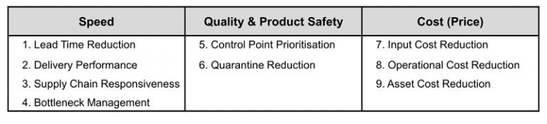
Speed

Another word for speed (as it relates to a supply chain) is throughput, or the pace at which profit flows through the supply chain.

Sales and marketing have a lot to do with this. Selling many widgets for many times their cost is always a great way to fulfil the need for speed! Hence, effective communication through a comprehensive S&OP system is vital.

The S&OP process can be used to monitor the impact of changes at 4 operational leverage points within the supply chain that help the sales and marketing guys increase speed.

1 - Lead Time Reduction

Lead times can be reduced in 3 ways:

Inventory Positioning– positioning inventory so that it is as close as possible to the customer is an obvious way of minimising lead time. Inventory can also be positioned to take advantage of the variability-smoothing benefits of stock aggregation (see What is Stock Aggregation and how can it benefit my supply system?). Both inventory positioning goals can be achieved by modifying an existing network or designing a completely new network.
Pipeline De-coupling – strategic, demand-driven inventory buffers can be used to achieve a combined benefit of decoupling parts of a pipeline, increasing inventory turns and reducing the leadtimes as seen by the customer. This approach can reduce inventory by up to 30% for make-to-stock positions. Refer to What is the demand driven approach to inventory buffer sizing? for more details on how to set up these strategic inventory buffers.
Supply Frequency– complex processing factories are now using a fixed-cycle-variable-volume load levelling technique, called a Product Wheels, to optimise order sizes, increase order frequencies and reduce lead times. The Product Wheel design process is used to make run length vs inventory vs lead time vs factory capacity trade-offs. See 7 essentials of a process factory scheduling cycle below, for more information on Product Wheels.

2 - Delivery Performance

Delivery performance at a Control Point (see 10 high-powered building blocks that simplify the way you look at your complex supply chain above) is made up of 5 tactical “rights”:

Right quantity
Right product
Right place
Right time
Right quality

Delivery performance is calculated by multiplying the performance of these 5 Right measures.

The nemesis of delivery performance is variability of which there are 4 types:

Demand Variability
Supply Variability
Operational Variability
Managerial Variability

Variability can be controlled with the strategic placement and design of buffers.

There are only 3 types of buffer in a supply chain:

Inventory buffer
Time buffer
Capacity buffer

Once buffers are in place and delivery performance has stabilised at an acceptable level, improvements can be made to reduce the size of the buffers.

See 10 high-powered building blocks that simplify the way you look at your complex supply chain above, for more information on buffers, Control Points, and their broader supply chain implications.

3 - Supply Chain Responsiveness

A modern supply chain must be capable of responding to sudden disturbances. Often, this responsiveness is part of a business’s supply strategy and a point of competitive difference.

Sudden disturbances in a supply chain are different to the “common cause” variation experienced in a stable supply chain. Common cause variation can be described statistically and follow a normal probability distribution.

Sudden disturbances, called “assignable or special cause” variation, can push a supply chain system out of control and make it unstable. Examples of special cause variation in a supply chain can include:

a customer stock take error that causes a sudden demand spike
a sudden weather or public health event
an unanticipated order from a customer caused by a competitor’s short supply
an opportunity to take advantage of a spot buy of cheap inputs
a sudden factory bottleneck caused by poor equipment installation
an unforeseen quality issue requiring that inventories be rebuilt quickly

The extent to which a supply chain is responsive, and is capable of absorbing special cause variation, is determined by the extent to which buffers have been designed to flex (see the 3 buffer types above).

Here are 2 examples of clever buffer flexing that averted possible supply disasters:

A supply director is asked to respond to a 30% increase in customer demand after a competitor’s factory was demolished in a fire. In previous years the supply director had been careful to retain certain modular assets in the factory which were old and fully depreciated and yet still serviceable. Also, he had maintained a constant ratio of trained permanents and casuals which gave him the ability to flex crewing very quickly. These 2 factors, combined with the judicious increase in overtime, meant that the supply director could dramatically increase, or flex, the size of his capacity buffer and respond to the sudden increase in demand.
A customer stock-take error creates a 15% increase in demand on a 3rd party suppliers’ factory. The customer says that the shortfall must be replenished within 8 weeks. The 3rd party supplier’s production line is 90% utilised and supplier tells the supply director that they are unable to respond to the sudden demand increase. The supply director knows that she can flex her inventory buffer because this is a seasonal product and they use larger inventories in the peak season to manage demand (it is currently the low season).

Collaborating closely with the supplier and the customer, the supply director instructs her planners to reduce the number of product changeovers required at the supplier’s plant (i.e. increase the supplier’s capacity buffer) and to forecast the customer demand increase (surge) in 4 weeks. She also instructs her planners to immediately increase finished goods inventory (i.e. flex the inventory buffer) to dampen the demand surge, thus averting a supply disaster for the customer and securing a supplier of the year award.

4 - Bottleneck Management

A system to manage bottlenecks within manufacturing supply chains was designed in the late 80’s by Dr Eliyahu Goldratt and introduced to the world when he published his first book called, The Goal, in 1984. This system is known as the Theory of Constraints (TOC).

Goldratt was a physicist and he used his understanding of pure maths and statistics to create a logical approach towards supply chain management that went well beyond his many introductory business novels.

Almost any production operator can grasp the concept of bottleneck although the challenge lies in understanding how manipulating that bottleneck impacts the rest of the supply chain.

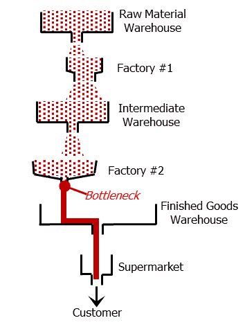
The picture below shows a healthy supply chain where the bottleneck is the customer.¹ This is the best place for a bottleneck in a supply chain because it ensures optimum delivery performance.

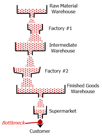
The important characteristics of a bottleneck are:

flow (speed) is slowed by the bottleneck
material accumulates before the bottleneck
downstream resources in the process are starved from supplies as the bottleneck cannot deliver enough to saturate them

To illustrate the behaviour of bottlenecks, and the nature of bottleneck management, we will show what happened to this supply chain.

The supply director was suddenly informed that supermarkets were threatening to de-list products from this supply chain because of exceptionally poor delivery performance. The supply director asked his planning team to represent the current state of the supply chain using simple funnels. With discussion it took them 15 minutes.

The supply director organised a teleconference with his team at Factory 2 and asked them to create a similar diagram for their factory, specifically in relation to the product that was at issue. 1/2 an hour later they produced the following diagram.

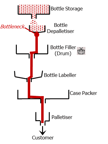
Another teleconference revealed that the bottle supplier for this product had been changed 3 weeks prior and the bottles had a high defect rate causing constant crashes at the bottle depalletiser (this is special-cause variation and meant the supply chain was now unstable).

The supply director marshalled his buying team into action and came up with a short- and medium-term strategy to rectify the situation. He also made a mental note to find a way of delegating and communicating bottleneck management.

For more information on bottleneck management in factories please go to our article – What is a flow line and how can it be manipulated to maximise performance?

Quality & Product Safety

The Six Sigma literature is a great resource for tools that help improve quality within a supply chain.

The challenge is to decide where to invest time, effort and resources using these and other quality tools.

There are 2 important quality related leverage points:

5 - Control Point Prioritisation

There are many operational Control Points in a supply chain (see 10 high-powered building blocks that simplify the way you look at your complex supply chain above, for more information on Control Points).

There are 2 tools that can be used to identify those Control Points that must be bolstered with additional quality analysis and monitoring. Both rely on marketplace and customer preference data:

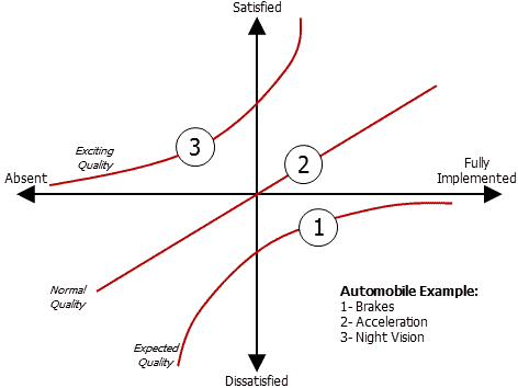
Kano chart – customer preference data (from warranty logs, customer complaints, call centre logs, etc) can be classified by plotting it on a Kano chart. The graphic below² shows a sample Kano analysis from the car industry. In this example, 3 customer requirements are identified for the automobile:

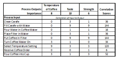
Cause-and-effect matrix – this is a way a capturing those points in a process that are the most important from a customer quality perspective. The graphic below² shows an example of a cause-and-effect matrix (for coffee at a truck stop). Processes with the highest correlation score have the strongest relationship to customer needs.

6 - Quarantine Reduction

The process industry generally, and food manufacturing specifically, often quarantine finished product to check a vital quality aspect of the product (e.g. seal integrity and therefore potential product spoilage at a food manufacturer) after a prescribed incubation period and before release to good stock.

Encouraging a reduction in allowable quarantine levels forces good minds to come up with ways of controlling the process more reliably at the source (e.g. in this case the process that creates the seals).

Instigating a statistically valid process monitoring system such as a traffic light system at the crucial process (e.g. sealing machine) has several benefits:

the incubation quantities can be scaled back according to the traffic light status at the time of production
traffic light systems give immediate quality feedback to the operators at the machines
a culture of right-first-time is reinforced
inventory carrying and logistics costs associated with the quarantined product are reduced
quality personnel are lees involved in administrating the quarantine system and can provide more assistance with root cause analysis creating a virtuous circle.

Cost (Price)

Costs are obvious, cost relationships are not so obvious. A glance at the APICS Supply Chain Operations Reference (SCOR™) framework² below shows how intertwined supply chains are and how exposed they are to weakening when anyone takes a one dimensional view. For example, if reducing costs also reduces speed and quality then this must be recognised and trade-offs understood and negotiated throughout the supply chain.

7 - Input Costs

Whether purchasing a commodity for internal supply operations or purchasing a finished product from an external manufacturer, purchasing managers have a fantastic ability to enhance or cripple a supply chain.

The purchasing managers that cripple a supply chain are the ones that focus solely on;

consolidating volume
negotiating minimum price

The purchasing managers that enhance the capability of a supply chain have these skills AND add maximum value by using:

Interpersonal skills (handling people, having respect for others’ opinions)
Team skills and facilitation (knowing when to be the leader and when to be the adviser)
Analytical problem-solving skills (translating knowledge into a total supply chain total cost-to-serve evaluation)
Technical skills (supplier relationships in the process industry are (should be) longer because supply chain optimisation in the process industry is driven by process improvements)
the list goes on (commercial acumen, computer literacy, ……)

The role of purchasing manager in the process industry should be extremely complex and extremely important and resourced with that in mind.

8 - Operational Costs

There are many initiatives within a business that reduce operational costs from minimising waste in transactional processes (e.g. accounts payable) through to reducing manufacturing costs.

The biggest impacts on logistics costs (such as transport, warehousing, and storage costs) are usually delivered through network restructuring supported by supplier and customer collaboration.

Manager’s searching for conversion cost savings at internal or external supply facilities rely heavily on broad-based continuous improvement systems with a focus on initiatives such as:

De-bottlenecking and buffer adjustment
Downtime reduction/efficiency improvement
Capacity improvement
Lean/Six Sigma
Pack/input consolidation and optimisation

This can lead to much wasted effort when these initiatives cannot point to broader supply chain benefits (see Modify the Lean, 6 Sigma and Theory of Constraints methodologies for your complex process factories below).

Also, costs within a complex factory, particularly the type found in the process industry, are not completely variable. There are usually cost thresholds that need to be breached to deliver savings and gradual improvements such as downtime reduction and efficiency improvement should be pursued with this in mind.

Here’s an example to illustrate.

Below is a Gantt chart showing a standard production week derived from a Product Wheel (see 7 essentials of a process factory scheduling cycle below for more information on Product Wheels) for a processing line. The supply team decided to make (what was) a broad-based continuous improvement effort more focused and outcome driven.

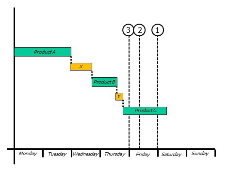
The team decided to increase the instantaneous capacity and running efficiency of products A and C as well as reducing the time taken for changeover X. They have communicated to the business that they will deliver cost savings as they pass through cost thresholds 1 thru 3:

Threshold 1 – Casual labour reduction because of not supporting the Saturday shift

Threshold 2 – Maintenance overtime reduction as the production line is made accessible on Fridays

Threshold 3 – Inventory (cash) and warehouse cost reduction provided by the ability to increase the number of changeovers on the line.

The team decided to cease all work currently underway on reducing the time taken on changeover Z because it was not even required on the standard production schedule (i.e. it was not required for the Product Wheel).

9 - Asset Costs

Customer’s focus on Speed, Quality and Costs (Price) whereas owners of the business (arguably the most important people) focus on the Return on Total Assets employed.

Current assets, mainly the cash tied up in inventory, is often viewed with ambivalence. Reducing inventories can cause a short-term reduction in profitability and a reduction in the recoveries at internal and external supply locations.

However, broader collaboration between supply sources and network managers, as well as some short-term fiscal pain, can lead to longer term cost reductions as the pipeline becomes more efficient and better aligned with demand. This in turn drives reduced expedite related expenses as well as reduced warehousing and logistics costs.

Finally, fixed assets always benefit from a customer focus. Increasing Speed (i.e. the pace a which profit flows through the business) improving Quality and reducing Costs, while using the same fixed assets, will always increase the return on fixed assets. This is a great virtuous circle and we will talk more of this later.

Now to think about how process factories are different from car factories where a lot of the current improvement systems were developed.

¹ – the credit for this diagram goes to Philip Marris, founder and owner of Marris Consulting, France.

² – taken from Supply chain excellence: A handbook for dramatic improvement using the SCOR model, P Bolstorff and P Rosenbaum, 3rd Edition. AMACOM 2012.

Step 2 - Understand the 7 fundamental differences between process factories and car factories

Lean manufacturing was developed using the Toyota Production System. Hence it is instructive for those working in the process industry to examine how process factories are different to car factories.

This understanding helps us make the necessary adjustments to packaged improvement systems (e.g. 6 Sigma) that have been developed with the car and the parts assembly industries in mind.

We have included the 7 fundamental differences below and you can also download this pdf that goes into more detail.

A production line should be designed with the intention of providing a quality product in a timely and competitive fashion. The car and process industries approach this goal in distinctly different ways.

1 – Line Design

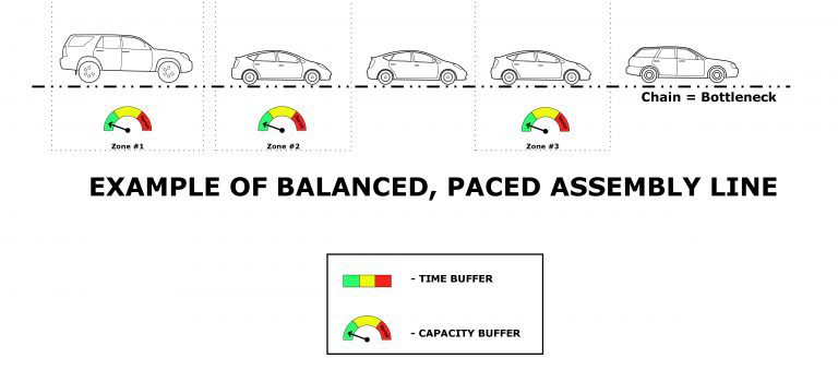
The car industry uses paced assembly lines. In a paced assembly line, cars flow through the line on a chain that moves at a constant speed. The cars move through zones that usually contain one or more operators. The line is designed so that the operators will almost always be able to complete their task while the part is in their zone. The bottleneck is the line-moving mechanism itself, the chain.

The process industry uses flow lines (although abattoirs are exception to this rule). In a flow line the stations are independent. Each station operates at its own speed, so the bottleneck is the slowest station in the line.

The car industry can strive for “one piece flow” (one-piece being a single car) cost effectively with a big focus on chassis design and standardised parts across models thus maximising the flexibility of a line.

The process industry cannot cost-effectively achieve one-piece flow. In most cases, the number of changeovers required to achieve run lengths of just one carton of product would be ludicrous and un-competitive. The process industry must run to quantities that are determined by the individual demand and supply characteristics of each SKU (see 7 essentials of a process factory scheduling cycle below for more on this).

2 – Line Capacity

Paced assembly lines are balanced. That is to say that the pacing mechanism, the chain, determines the current capacity of all resources on the line. All workers must complete assigned tasks within the allotted pacing time. Capacity that exceeds the pacing mechanism is a waste.

Therefore “takt times” play an important role in the Toyota Production System. There is a lot of flexibility on a paced assembly line to adjust resources to cater to the different product requirements in the line while maintaining takt time.

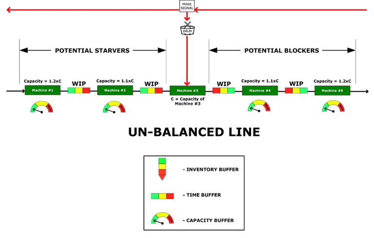
In a complex, high volume flow line (such as those used in process factories), the tasks depend more on the machines at each station than the people supervising them. The cost of capacity is typically not the same at each station, so it is easier to maintain excess capacity at some stations than at others.

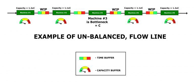
Flow lines therefore are often un-balanced with additional capacity upstream and downstream of a distinct bottleneck (usually the highest cost machine). This additional capacity shields the bottleneck from starvation and blocking, see the next graphic.

The optimum operation of an un-balanced flow line is a function of the statistical interplay of capacities and Work in Progress (WIP). See What is a flow line and how can it be manipulated for maximum performance? for more information on this topic.

3 - Role of Operators

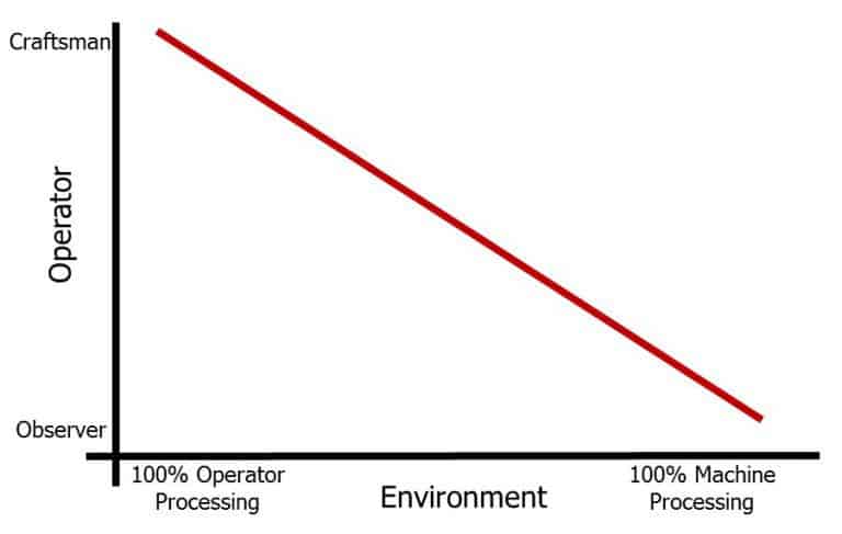
Operators on a paced assembly line interact with the product. The quality of the output from their zone is much more dependent on their physical skills and the way they manage their resources, such as parts. They are more craftsmen than observers.

Operators, on the type of high-speed flow lines used in the process industry, have a limited ability to interact with the product. In high speed food production for example, the product itself can be invisible to the operator. While they can influence the performance of their line with knowledge, their role is more observer than craftsman.

There is always an upper threshold of performance that can be achieved on a flow line by improving operator skills and motivation alone. That threshold is determined by the design of the flow line and the distribution of capacities and WIP.

4 - Management of WIP

Paced assembly lines are regulated by the pacing mechanism so the WIP (in terms of cars) is equal to the number of cars on the chain. It takes 20-30 hours to build a car (i.e. value-adding time) although a single car can be on the paced assembly line for 2-4 days. A parts WIP is also used at the work zones to shield the assembly line from short term delivery risks for inbound parts. Kanban cards are used to control WIP levels.

Flow lines used in high rate processing factories use WIP for the following reasons:

Shield the bottleneck
Absorb upstream sequencing and changeovers
To facilitate processing needs such as cooking, brewing, maturation, etc
To shield equipment from short term delivery risks for inbound materials

Value-adding time (by machines) for high speed flow lines in the process industry, is usually less than 1 minute and this is only exceeded where there are product maturation requirements (e.g. enzyme reactions for flavours). Total time in the production line can be affected by sequencing needs although this rarely exceeds 12-14 hours. In a flow line, WIP and machine capacities can be manipulated cleverly to achieve optimum total line efficiency and throughput.

Unfortunately, the notion of balancing a line has become so ingrained from Lean proponents and from paced assembly line environments, that it is often applied to flow lines in the process industry which is inappropriate and counterproductive. Again, see What is a flow line and how can it be manipulated for maximum performance? for more information on this topic.

5 - Application of Improvement Methodologies

The number one issue with paced assembly lines is time. Lean principles are heavily laden with a focus on minimising the 7 wastes which focus directly, or indirectly, on time. Also, one of the foundation Lean tools is 5S which is imminently applicable in paced assembly lines where operators must manage their environment in a time critical way.

Time is also important on Flow Lines but ONLY AT THE BOTTLENECK. The performance of flow lines used in the process industry rely more on the complex interplay of capacities, WIP and efficiencies and how these characteristics can cost-effectively optimise performance at the bottleneck.

Also, the performance of a flow line used in a process factory is a trade-off between maximising flow and dealing with the complexities of what is essentially a “live” material (see point 7 below for more on this).

Often, the blind application of Lean tools in process environments can deliver lacklustre results. For example, application of 5S in a processing environment, while beneficial from a cultural point of view, can deliver very little operational benefit in a factory that is already heavily regulated from a food safety and hygiene point of view.

6 Sigma tools have much more applicability in processing environments, when compared to Lean tools, particularly since success with flow lines has more to do with the statistical nature of performance. Like any tools though, they must be prioritised and applied with discernment and this can be difficult to achieve in complex flow lines.

6 - Value Stream Mapping

If you review the literature on value stream mapping, then you will probably find only 3 books of any value (published by the Lean Enterprise Institute):

Learning to See (1999) – single plant (door to door) value stream mapping – Case study used in book = Steering bracket manufacturer
Seeing the Whole Value Stream (2003) – factory to factory (extended) value stream mapping – Case study used in book = Wiper blade manufacturer
Building a Lean Fulfillment Stream (2010) – supply chain (dirt to customer) fulfilment stream mapping – Case study used in book = Air conditioner manufacturer

The ideas in these books have been manipulated over the years (often with questionable technical rigour) to suit different industries. The books are tailored towards supporting the car industry with an obvious influence from paced assembly lines and therefore a strong focus on time.

Value stream mapping can be applied to the flow lines used in the process industry however, they must be modified to take account of the un-balanced nature of the capacities found along almost all flow lines. This is a weakness in the value stream mapping techniques shown in these books.

As if to prove the point; unfortunately the steering bracket example shown in Learning to See is actually an un-balanced flow line and when a more thorough capacity analysis is done on this line it shows that it is out of capacity by 10% relative to quoted demand, a significant waste not identified by the standard value stream mapping approach.

7 - Load Levelling

There are three parts to levelling the production load at a manufacturing facility:

Level the demand – minimise variability and associated bullwhip effects on demand signals.
Level the production mix – rotate through products as quickly as possible. The more you level the product mix at the bottleneck process, the more able you will be to respond to different customer requirements with a short lead time while holding little finished goods inventory.
Level the production volume – create a consistent production pace or cadence at the bottleneck which is a good representation of customer demand/pull.

The extent to which the production mix and production volume should be levelled is determined by a trade-off between the cost of changeovers, the cost of inventory and customer delivery performance.

A paced assembly line is well suited to load levelling. Car models and variants can be spread across the pacing mechanism (the chain) according to mix and volume. Each operator zone can be tailor-made to adjust (changeover) very quickly between models and variants. The Hiejunka Box (or at least the thinking behind it) is a Lean tool used for load levelling that can be applied to paced assembly lines.

High speed flow lines used in the process industry are an entirely different operating platform. For example, if it takes a 2-hour stoppage at the bottleneck to Clean In Place (CIP) between certain products then it doesn’t make sense to run these products for only 10 minutes. This is an example of a physical and microbiological reality that must be faced in a pragmatic way.

Load levelling for flow lines in the process industry can still be achieved using a technique called Product Wheels developed by Dupont™ and Exxon. Product Wheels are a Fixed-Interval-Variable-Volume load levelling technique and are the domain of a plant scheduler (not a Hiejunka box). Refer to the next chapter for more information on this technique.

In fact, the quest to replace a plant scheduler with a computer in the process industry has been the challenge of many a statistician or computer science devotee. The “scheduling problem” for this type of environment is recognised as one of the biggest challenges for computer power … still.

Anyway, the schedules and sequences used by the process industry can usually be levelled using a standard Product Wheel of about 3 weeks in duration. There are many factors to consider when designing and optimising a Product Wheel for the process industry which can include (but are not restricted to):

Sequence restrictions caused by contamination issues (e.g. colours, salt levels, trans fatty acids)
CIP and food safety requirements (e.g. allergens, statistical inspections)
Coordination of intermediate product storage and blending
Sequence restrictions caused by product requirements (e.g. Halal, etc)
Variation of process and equipment capability between products (e.g. maximum product temperature)
Sequence rules used to minimise cumulative changeover time.
Sequence rules used to avoid resource clashes (e.g. equipment, labour skills, etc)
Sequence restrictions caused by product design (e.g. tainting caused by fish)
Sequence impacts of packaging design (particularly shelf-ready packaging)

So …….. what do these “Product wheels” look like ……… read on!

Step 3 - Identify the 7 essentials of your process factory scheduling cycle

A good quality factory schedule is one of the most important factors in minimising costs and creating a firm foundation for continuous improvement. Yet many factory schedules are driven by the knowledge of just one scheduler, without much oversight by senior production management.

In this section we will explore the important parts of a scheduling cycle and provide a few rules of thumb for process factories.

Note: If you don not think you have a standard scheduling cycle (i.e. a template that is used periodically by a scheduler to rough out a new scheduling cycle) then just ask the scheduler. If it is not documented, then it’s probably just locked away in the schedulers head.

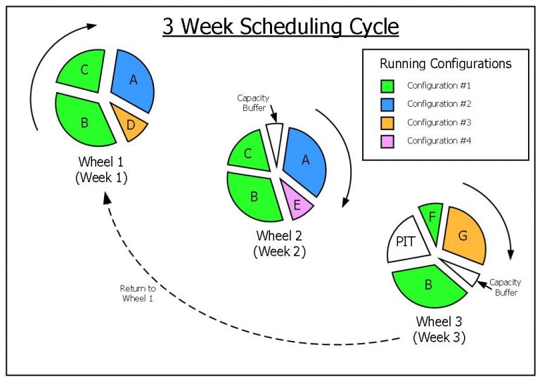
1 - Recurring Cycle

Product portfolios in the process industry are complicated. Paradoxically this makes it easier to create a recurring scheduling cycle for a given production line. If different and complex products are always required to run on the same complex processing line, then there is always a logical way to order these product runs (see next heading). If the average demand for each product is also calculated it becomes a matter of desk work to create several weekly cycles as shown below.

These are known as Product Wheels and in the process industry there are usually 3 or 4 weekly Product Wheels in a standard recurring scheduling cycle.

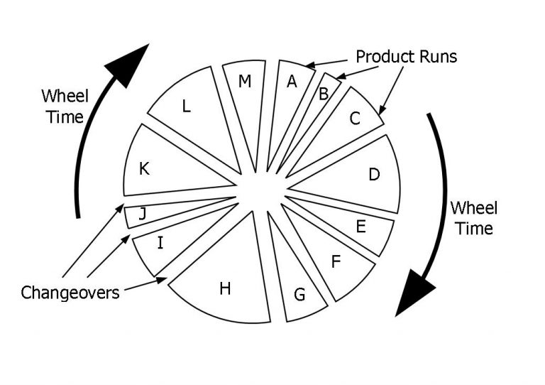
2 - Product Runs

The duration of each product run is simply the instantaneous rate at the scheduled machine on a processing line multiplied by the average running efficiency.

The instantaneous rates used in production schedules are notoriously wrong and yet they are often easy to ascertain. They run afoul of a view that they should be made “stretching” when the reality is that instantaneous rates in complex processing environments are more a function of equipment design than employee training or motivation (although obviously people management is an important enabler for production performance).

Running efficiency is different to Overall Equipment Effectiveness (OEE). Running efficiency excludes variables such as changeover times and line availability. Running efficiency is easy to calculate with enough historical product run data. It is simply cartons produced divided by the cartons that could have been produced at the maximum instantaneous carton rate.

In the process industry there are up to 250 product runs in a recurring, 3-week schedule cycle. The duration of each product run can be anywhere between 30 minutes and 6 hours.

3 - Running Configurations

Each processing line usually has between 15 and 30 ways it can be set up or configured. These are known as running configurations.

Each product run is aligned with a single running configuration. But one running configuration can be used for many different product runs. As the Product Wheels above demonstrate, one running configuration can often account for a disproportionate volume of product (see Running Configuration #1 in the graphic above).

In fact, the most important running configuration on a processing line will usually account for over 40% of the total time in a recurring cycle. It follows that it is extremely important to know this running configuration intimately and concentrate on its improvement.

4 - Changeovers

Changeover time is that time taken to change from one product run to another. The time is measured at the scheduled machine.

All changeovers are not created equally. It is usually an easy task, once the standard Product Wheels have been defined, to list the frequency and duration of each changeover according to the “from” and “to” products.

If there are 50 changeover types in a recurring cycle, then usually the top 4 changeover types (as determined by the “from” and “to” products) will account for 30% of the total changeover time. It is important to concentrate on improving those changeovers that contribute the most lost time in a Product Wheel.

Total changeover time in the process industry accounts for approximately 10% of the total recurring cycle time.

5 - Sequence

If you need to run say a black and a white product within a recurring cycle, then it makes sense to run the white product first to minimise the cleaning and changeover time.

If, out of say 50 changeover types (see above) on a production line, there are 2 or 3 changeovers that are exceptionally long then it makes sense to always do these changeovers during Process Improvement Times (see below).

These are just 2 examples of the way the characteristics of products or processes determine the sequence that best suits a product portfolio. Schedulers always run to a sequence (whether they can articulate it or not) and that has usually developed with many interactions with senior production employees.

There are huge cycle time benefits to be had by formalising and optimising the sequence used in a recurring schedule cycle.

6 - Process Improvement Time (PIT)

Process Improvement Time can include any or all the following

Improvement team activities
Maintenance
Cleaning
Off-line set-up
Meetings
Team building

7 - Capacity Buffer

Finally, there needs to be an allowance for variability; both supply (factory) variability and demand variability.

Some managers deny that any allowance needs to be made for supply variability but data from many factories shows that for a medium technology factory with an average reliability there is about 10% variability against schedule target for each product run. That is to say that actual production can be 10% greater or 10% less than the original scheduled target for a single product run.

The good news is that if there are 10 or more product runs in a row then we can apply some statistical tricks. The variability of this total group (i.e. > 10 product runs in a row) is half the variability of the single run or 0.5 x 10% = 5%.

If we assume a similar variation for demand, we get another 5%.

Finally, we can apply a safety factor of say 50% for Murphy’s law so our total capacity buffer would be (5% + 5%) X 1.5 = 15%.

So, we have created Product Wheels and optimised them in relation to inventory, changeover costs and performance. We have used something called Running Efficiency rather than Overall Equipment Effectiveness (OEE) to determine line behaviour.

The question is whether OEE still plays a role and whether it is the right performance metric for the process industry.

Step 4 - Monitor the best top-level performance metric at your process factories

Overall Equipment Effectiveness (OEE) is often used as the main metric for factory performance in the process industry (food & beverage, liquids, sheet goods, solid & fluid packaging operations).

However, while OEE is a good measure for independent workstations and processes, production lines in the process industry are usually made up of several workstations and processes which are all connected, rendering the traditional OEE metric less than ideal.

Before we come up with a better metric let’s first review the origins of the OEE metric and define how it is calculated.

The OEE metric was made famous by the Lean movement although it originated from the development of Total Productive Maintenance (TPM). TPM evolved from the parts manufacturing and assembly industry in Japan. Its parallel evolution with the Toyota Production System during the 1950’s thru 1960’s makes TPM, and therefore the OEE metric, intimately linked with Lean.

The graphic below shows the building blocks of the traditional OEE measure.

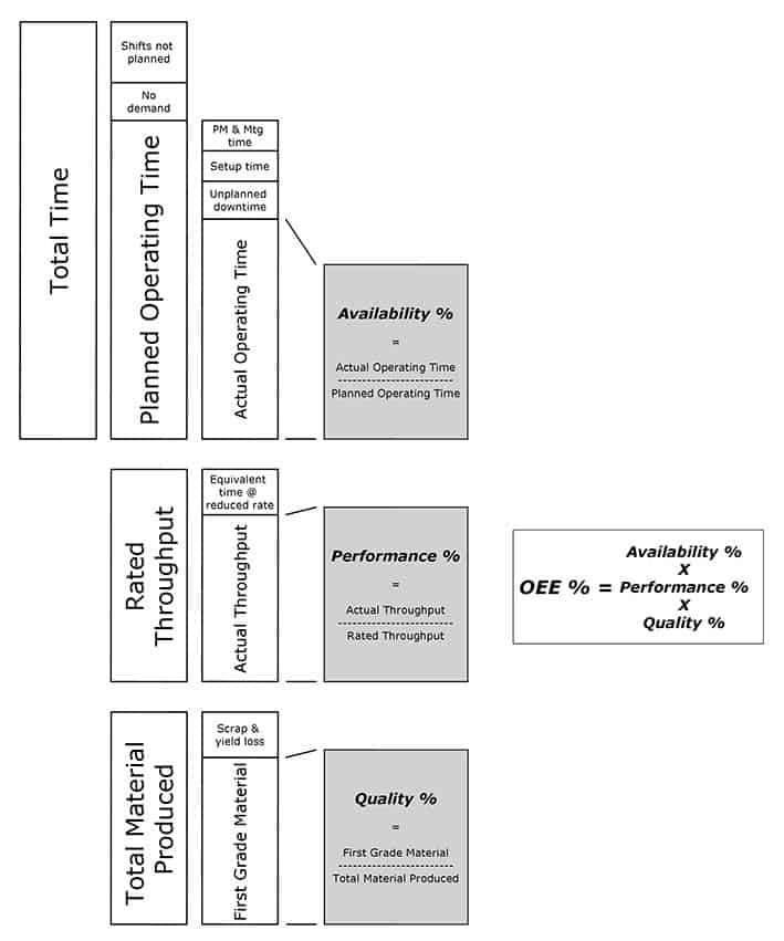
OEE was developed with discrete workstations in mind such as lathes, assembly stations, robot stations, etc.

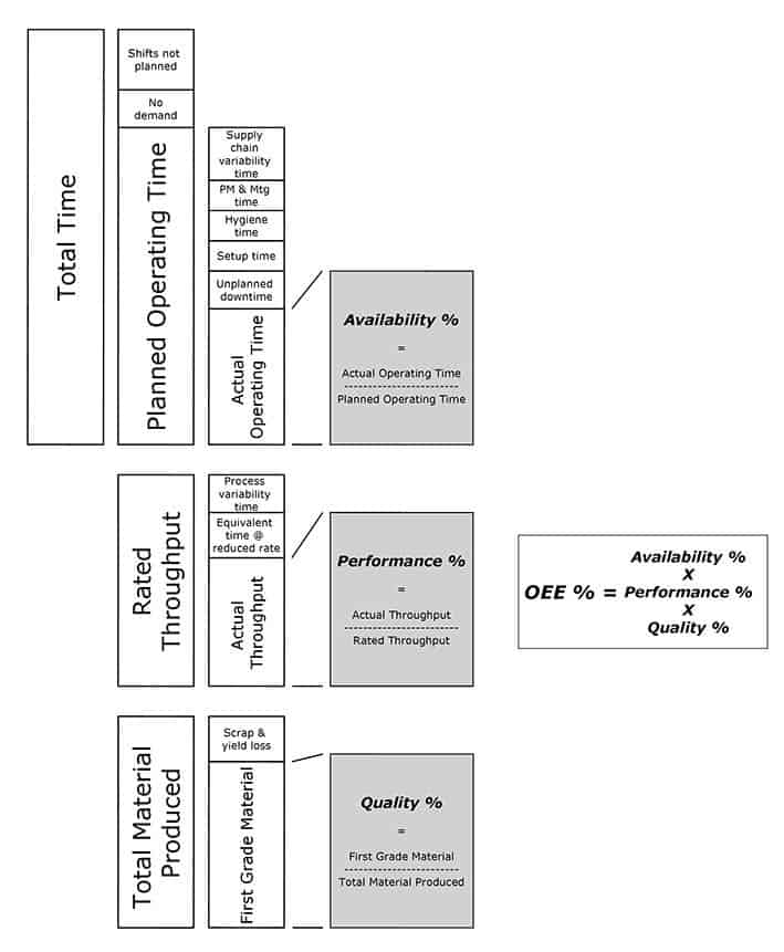
The challenge for the process industry is to develop an OEE-type measure that can be used for entire production lines or factories that are made up of interconnected workstations or processes.

First, we need to deal with a couple of characteristics of entire production lines or factories in the process industry.

Setups in the parts manufacturing and assembly industry relate to the physical changeover of equipment. An OEE-type metric for the process industry must incorporate the impact of hygiene (cleaning) time as well as physical setup time.
All factories are part of a total supply system and so the OEE-type metric for production lines and factories must deal with need to “store” capacity in the form of supply chain variability time and for (factory) process variability time. That is, we need to put time buffers into the system (see Introduction).

Therefore, we need to modify the traditional OEE calculation to encompass these 2 issues as shown below:

Now, let us assume that we have a straight-forward processing line (like the one shown in the graphic below) and we want to stick with the traditional OEE measure above. The only way we can do it is to measure performance at the bottleneck, shown below as machine #3 (the Drum).

We might be able to get most of the data for the traditional OEE measure however, we will struggle to record accurate “unplanned downtime” and “equivalent time @ reduced rate” information at the bottleneck.

Unplanned downtime at the bottleneck could have been caused by the reduced rate of equipment upstream or downstream of the bottleneck. Conversely, reduced rate at the bottleneck could have been caused by the unplanned downtime of equipment upstream or downstream of the bottleneck.

Splitting these 2 metrics is complicated and so for the sake of simplicity it would be helpful to combine these measures into a Total Unplanned Downtime measure.

But this would mean combining the Availability and Performance components of the traditional OEE measure and potentially create confusion for the purists!!

That’s it!!! ……. we need a new measure for the process industry!!! …… no wait …. maybe not.

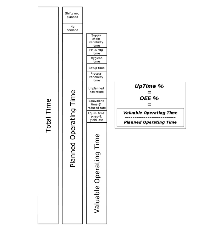
There is another calculation accepted by the Total Productive Maintenance community called UpTime which gives the same numerical results as OEE for a given line, is easier to understand, includes all the constituents of the OEE measure and allows us to combine “unplanned downtime” and “equivalent time @ reduced rate” into a single measure.

This is all summarised in the next graphic:

So, before we finally combine the unplanned downtime with the equivalent time @ reduced rate measures, let’s just clarify further why it is helpful to create one total downtime measure for inclusion in the UpTime metric.

As stated earlier, process lines and factories in the process industry are made up of interconnected workstations and processes, directly coupled using conveyors, pipework and pumps, hoppers, etc.

In these situations, the joint OEE (= joint UpTime) for a system of directly connected (non-buffered) processes reduce as the number of interconnected processes increases.

The graphic below shows what happens when workstations or processes, which by themselves have an independent OEE of say 80%, are connected together without buffering.¹

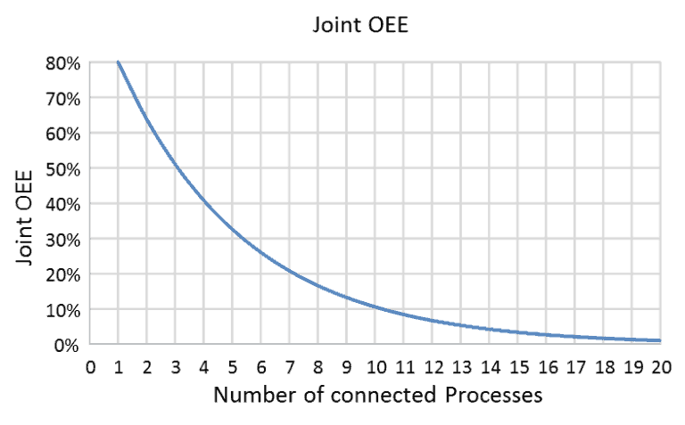
In the process industry it is common to see 5 or more interconnected workstations or processes. In these cases, managed buffers (in the form of time (WIP) and capacity buffers) are used to create un-balanced flow lines as shown in the process map below.

These un-balanced flow lines help to support joint OOE’s (= joint UpTime) of greater than the 40% that would otherwise have been achieved. This is often the only way a high-technology line can be made financially viable.

We go into more detail about unbalanced flow lines in our article What is a flow line and how can it be manipulated to maximise performance? For this guide it’s enough to say that one of the processes is identified as the “Drum” and buffers are used to ensure that the Drum doesn’t get starved or blocked.

The extent to which this is actually achieved, and therefore the joint OEE (= joint UpTime) as measured at the Drum, is maintained at an acceptable level (a good unbalanced line should have a joint UpTime > 70%), is determined by the statistical interplay of time and capacity buffers on the line.

However, the difference between “unplanned downtime” and “time @ reduced rate” at the Drum becomes less important and harder to attach a root cause. The unplanned downtime or the reduced rate could be caused by any one of the workstations. They could also be caused by the behaviour of the buffers.

The more useful measure is Total Unplanned Downtime (which incorporates unplanned downtime and time @ reduced rate) because this recognises that the statistical behaviour of the line is complex and there is no value in separating unplanned downtime and reduced rate. In both cases the result is the same, a reduction in valuable operating time.

Finally, the UpTime metric above is still a bit cumbersome and can be made more useful by introducing the terms Crewed Time, Usable Time, and Utilised Time, see below:

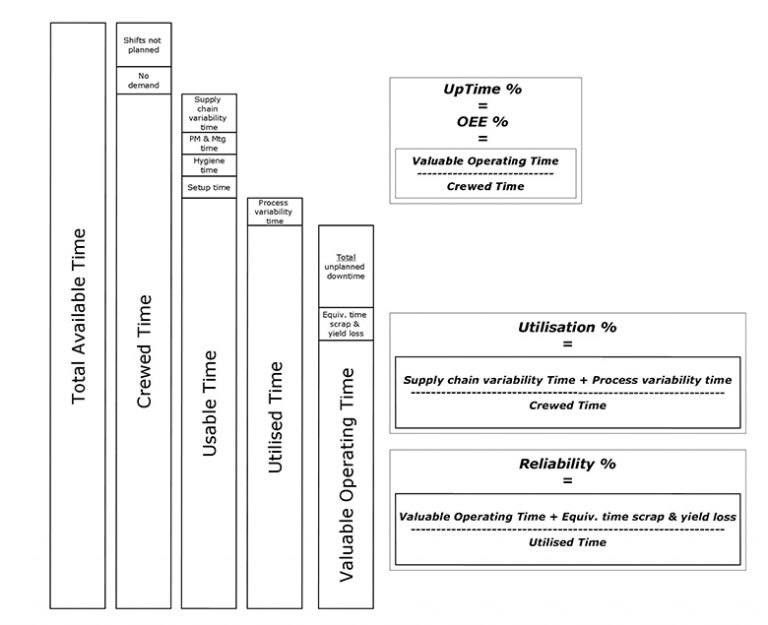
This allows us to establish 5 powerful measures (apart from UpTime) that define the asset performance of a total line or factory in the process industry (remembering that asset performance is the most important measure in the process industry);

1 – Crewed Time (% = Crewed Time/Total Available Time) – Some refer to this as “Lights-on Time”. It’s a measure of how much a line or process is required to be available to production to make product. If the Crewed Time is low, then the reason for the assets existence should be questioned. If two lines (capable of making the same products) have a Crewed Time of less than 50% each, then there is an opportunity for asset consolidation. We have seen Crewed Times as low as 8% on lines that are relatively high cost and still being depreciated. Crewed Time (and asset allocation) is the domain of senior plant management and schedulers and has a direct correlation with Return On Assets (ROA).

2 – Usable Time (% = Usable Time/Crewed Time) – Is a measure of how much the line time is tied up in setup, hygiene, and preventative maintenance time. It is a function of line design, number of products on the line and line scheduling. Highly technical lines with complex products will have a lower Usable Time when compared to a simpler line with only basic operational requirements. Also, the Usable Time will be greatly increased by a skilled scheduler that can manipulate the scheduled sequence to minimise total changeover times (e.g. running sensitive products with allergen claims before moving onto other products with less onerous cleaning and swabbing requirements).

3 – Utilised Time (% = Utilised Time/Usable Time) – The difference between Usable Time and Utilised Time is a measure of total process, line, or factory variability. If schedule attainment is measured over a period of say one week (in which say more than 10 different products are run) then this allowance is about half the variability of each run when compared to the average. So, for example, if a line has an average Reliability (see below) of 85% at +/-10% variability for each product then (over a period of a week) the schedule must allow an additional 0.5 * 10% = 5% for additional catch up time so that the customer is not short shipped.

4 – Utilisation (see graphic above) – Is a measure of how close the business can schedule a process/factory compared to planned demand and is a function of the historical variation in the supply chain and the process/factory. The variability allowances are larger (and therefore utilisation lower) for unreliable processes and for supply chains with poor demand forecasts.

Initiatives focusing on utilisation should focus on process reliability first before tackling the supply chain. Supply chain variability is best reduced by moving to pull systems rather than relying totally on forecasts (particularly in environments of ever-increasing demand volatility). A line/factory with utilisation more than 90% should generally be considered out of capacity unless there are robust reliability and pull systems in place.

5 – Reliability (see graphic above) – This is the measure that a maintenance manager should use to assess his or her performance. It is free from crewing, scheduling, and utilisation impacts that the maintenance manager cannot influence.

We get asked about reliability a lot so here is some more detail.

The derivation of Reliability for an un-balanced line is related to the extent to which the Drum process is blocked or starved. We have shown the diagram of our basic un-balanced flow line once more below:

We can make the following comments about Reliability for an un-balanced flow line:

Reliability for a total process/factory is a function of the efficiency of the Drum process and the extent to which the Drum process is starved (by the downtime or slow time of the upstream processes) or blocked (by the downtime or slow time of the downstream processes)
Theoretically, the Reliability of the entire line can simply equal the efficiency of the Drum process (in this case machine #3) if the time and capacity buffers are large enough to absorb upstream and downstream downtime and slow time.

The extent to which the Drum is impacted by starving and blocking behaviour can be calculated by monitoring the Control Points. For example, if the conveyor at Control Point C2 is empty say 40% of the Utilised Time for a certain product, then this helps to isolate the cause of Reliability issues as significant starving problems for this line when running this product.

Likewise, if the conveyor at Control Point C3 is full and stopped while the adjacent WIP hopper (time buffer) is also full for say 40% of the Utilised Time then this helps to isolate root cause as significant blocking problems.

Blocking and Starving behaviour on an un-balanced flow line can be quite complex and means that some downtime on the line (depending on where that downtime is located) is much more important that other downtime. This can make tools such as Pareto Diagrams (80-20 rule) less relevant.

So … we have dealt with the schedule and we’ve got a line or factory performance metric that is better suited to the process industry …… we are good to go!!!! ……. Not quite.

¹ – Taken from Christopher Roser’s site – allaboutlean.com

Step 5 - Introduce the 7 most important shop-floor metrics at your process factories

UpTime (which we argued in the previous step is a better performance measure for the process industry when compared to OEE) is a summary measure. While it is a strong indicator of factory or process performance, it does suffer from data latency and it does rely on data consolidation and averaging.

Consequently, by the time coal-face operations people see the latest UpTime results, they find it almost impossible to interrogate the data for root cause and create prioritised responses. The UpTime metric is best described as a “lagging” indicator.

In this section we identify 7 “leading” performance metrics for the people at the frontline of a process factory. Improvements in these “leading” metrics will will improve the “lagging” UpTime measure.

These 7 measures are in the order of priority as seen by the broader supply chain.

1 - Variability

The broader supply chain sees a factory as a black box that produces product. Variability and cycle time are really the only two performance metrics that supply chain managers get concerned about. All other metrics fall into the category of costs.

So, as long as the product is being supplied within agreed pricing terms, the other metrics are nice to know but not a concern for the broader supply chain (providing of course that those other metrics are not the root cause of increased variability or cycle time).

Over 95% of variability from a factory is caused by factory performance issues rather than raw material supply issues. This is because the buffers between raw material suppliers and the factory serve to minimise the flow-on impacts of raw material supply shortages.

Our experience is that a good production line and crew can achieve schedule targets within +/- 10%, providing of course that the targets are based on reality.

When a production crew falls short of a scheduled target, they invariably run longer to make up the shortfall. This relies on some confidence that they can make up time when they changeover to the next product.

This behaviour, along with some statistical benefits, mean that its better to measure variability over at least 10 production runs. Individual runs that have a variability of +/-10% usually smooth out to +/-5% over a 10-run group. +/-5% variability against an agreed schedule is usually a good target for the production folks.

2 - Cycle Time

Cycle time is the other metric that the broader supply chain considers. Cycle time (sometimes referred to as replenishment time) has the potential to improve supply chain responsiveness and minimise outbound stocks at this time of unprecedented uncertainty. This metric has the potential to do such good for the broader supply chain and yet we shake our heads at how few businesses, not just factory personnel, engage in its improvement.

A discussion about cycle time reduction in the process industry can be quite complex. This is because many different products, with different running characteristics, are run off the same line. So, optimisation of cycle time, with due consideration to total business costs, needs input from many stakeholders and can involve significant analysis work.

The good news is that the Product Wheels concept, discussed above in 7 essentials of a process factory scheduling cycle, can be used to help identify optimum cycle times across a product portfolio on a process line.

3 - Capacity and Utilisation

Factories in the process industry should not be more than 85% loaded within an S&OP planning horizon. 15% is generally the minimum capacity buffer required to absorb demand variation, inbound raw material variation and factory performance variation. It should be said that overtime shifts, deployment of discretionary labour (e.g. casuals) and crew allocation adjustments (e.g. stopping a line to run another) are all valid forms of capacity buffer but these are levers that should be managed carefully to minimise costs.

The capacity of a line is determined by how a business has chosen to crew it. So, for example, a line can be 85% loaded but run only on an 8 hour day shift, 5 days per week. In this case the utilisation of the line is only 24%. Utilisation is a measure of asset performance so any discussion about capacity should also be had in the context of utilisation to ensure robust business plans are made.

Capacity and utilisation metrics and targets could be used on the factory floor and yet most of the time these are hidden. This is because senior managers often fear complacency if too many production personnel could understand the existence of capacity and time buffers. Better to let everyone think that all lines are at maximum capacity (without discussing utilisation) and focus on 4, 5, 6 and 7 below. The jury is still out on this one.

4 - Rate

The achievable instantaneous rate for each product at the scheduled machine should be defined and monitored. Often production personnel are unsure of the scheduled machine let alone the scheduled instantaneous production rate for each product.

5 - Efficiency

Efficiencies that matter are those measured from the time a line is asked to perform at a certain consistent, instantaneous rate until when it is stopped in order to undergo a changeover of some sort or a planned adjustment or intervention. This “Running Efficiency” target will change between products and different line configurations. These Running Efficiencies should be measured and targeted.

6 - Changeover Time

In the process industry it is unusual to see cumulative changeover times exceed 15% of total crewed time for a line.

Also, in the process industry, changeover times are a function of line design. The changeover time is dependent on how the line was configured before the changeover and what the configuration needs to be after the changeover.

Our experience is that there are usually only 2-3 from-to line configuration changes that make up over 50% of the total changeover time on a line. These should be known, monitored and improved.

7 - Planned Time

Planned time is simply any activity, other than running or changeovers, which occurs while a line is crewed. This can include start-up preparation, clean-in-place operations, maintenance activities (not including breakdown/reactive maintenance), etc.

Planned time in the process industry is almost entirely a function of line design. It usually constitutes around 5% of total crewed time and can be influenced by better scheduling, continuous improvement activities and operator training. In any case, total planned time is worth having as a KPI.

OK, so you might be convinced about the difference between a process factory and a car factory. You might be sold on the arguments around schedules, line metrics and factory-floor metrics. But I can hear you cry .. what about my Lean (6 Sigma or Theory of Constraints) system ……. it must be worth something!?

The answer is yes, it is worth something …. but it could be worth more.

Step 6 - Modify the Lean, 6 Sigma and Theory of Constraints methodologies for your complex process factories

The process industry (food & beverage, liquids, sheet goods, solid & fluid packaging operations) differs from the car and parts manufacturing and assembly industry, where the Lean, 6 Sigma and Theory of Constraints methodologies were developed.

From the previous sections you can see that the unique characteristics of supply chains in the process industry make them less responsive to a one-size-fits-all approach. Performance optimisation in the process industry requires a customised approach.

We now move through the 3 key considerations when modifying the Lean, 6 Sigma and Theory of Constraints methodologies for the process industry:

The structural differences
The good
The not so good

The Structural Differences

At the macro level there are 5 structural differences between the process industry and the car and parts manufacturing and assembly industry that effect the way an improvement platform should be designed and implemented (see Step 2 – 7 fundamental differences between process factories and car factories for a more detailed comparison);

1. Labour Percentage – Using round numbers, in the parts manufacturing and assembly industry, labour is 70% of the factory cost; material and capital form the other 30%. In process industries, the ratios are reversed. Labour represents approximately 30% of the cost of manufacturing; capital and materials represent the other 70%.¹This puts a heavy burden on management in the process industry to ensure that improvement initiatives utilise labour more effectively and convert continuous improvement involvement into bottom line results.

2. Waste Accumulation – the manufacturing process in parts manufacturing and assembly often has many small and separate steps resulting in small accumulations of inventory, transport, or other forms of waste between the steps. Automated lines in the process industry rarely have discontinuities that cause uncontrolled accumulations of material between steps. Waste accumulation in the process industry usually takes the form of stand-by labour or capital.

3. Line Design – In the parts manufacturing and assembly industry manufacturing lines can be balanced using labour. If there is a short term capacity mismatch caused by breakdown losses, then workstation capacities can be adjusted by adding labour or other resources.

High-tech processing lines rarely have this labour-flexing capability and so automatic managed buffers are used to absorb downtime losses which creates un-balanced flow lines (see graphic below and What is a flow line and how can it be manipulated to maximise performance? for more information on un-balance flow lines). Un-balanced flow lines have an upper threshold of performance which is determined more by the statistical interplay of machine capability and managed buffers and less by crewing and training.

4. Operator interaction – Operators in the parts manufacturing and assembly industry interact with the product on a much more intimate level. Product quality and production capacity are influenced more by their training and the way they manage their resources. They are more craftsmen than observers.Operators in the process industry have a very limited ability to interact with the product. While they can influence the performance of machinery using their knowledge, their role is more observer than craftsman (see graphic below).

5. CI resource & training strategy – The small flexible accumulations in parts manufacturing and assembly environments alert operators or managers to the presence of small problems in their operation. Enabling many people to address many small problems is a powerful force multiplier and general “Continuous Improvement (CI)” training can create a powerful virtuous circle.

The statistical, high-technology, capital intensive nature of processing environments makes the efficacy of general CI training less influential on the bottom-line. CI training can establish a sound base of knowledge although that knowledge most be directed in a forensic way. Therefore the CI resource and training strategy for the process industry contains many more subject matter experts, individual contributors, mentors, technologists, and analysts.

The Good

The Big 4 improvement programs; Lean, 6 Sigma, Theory of Constraints and Total Productive Maintenance are applicable to the process industry with some modification and nurturing.

See these articles for more information on the applicability of each improvement system to the process industry and how each one must be modified:

It is GOOD to have consistent approach to your improvement platform although it is not important to align yourself with just one approach. In fact each of the Big 4 has a focus:

Lean – common sense tools for waste removal
6 Sigma – technical tools for variability reduction
TOC – common sense and technical tools for bottleneck removal and system optimisation
TPM – the maintenance “arm” of the Lean movement

A customised improvement platform that cherry-picks the best of the Big 4, selected on the basis of the unique needs of your operating environment, is the best way to go. This is particularly true for the process industry.

Setting up an improvement platform for the process industry is good for 5 reasons:

Culture – most operators in the process industry are observers, see above, and lets face it this can be boring! Creating a culture of improvement using an overarching program is helpful in creating employee engagement, demonstrating that the business is interested in improving work environments and offering employees a way of engaging with the broader business.
System – labour percentages in the process industry are much lower than the parts manufacturing and assembly business so creating a systematic and efficient way of driving improvement through precious and limited resources is worthwhile.
Training – all of the Big 4 tools can be supported by structured training programs although, for the process industry, tools must be selected wisely (see links above) and training should incorporate a strategy for subject matter experts, individual contributors, mentors, technologists and analysts.
Common language – the names of most of the tools used in the Big 4 improvement programs are widely used throughout manufacturing industry. So sticking with these tools helps to promote a common language, makes the skills transferable across business units and helps with the credibility of the improvement effort.
Springboard – creating the improvement platform with all the systems, procedures and training creates a springboard for many future change initiatives that need to be introduced to a production platform. It offers a ready-made system for disseminating and receiving information, distributing training, and eliciting operator engagement during projects.

But there are 5 vital ingredients that are missing from packaged improvement packages, which leads us into the not so good.

The Not So Good

There are some not so good aspects of packaged improvement programs and 5 of these are particularly true for the process industry:

Lack of priority – none of the Big 4 programs offer much help when it comes to the Industrial Engineering and Operations Research techniques needed to assign priorities to improvement activities. This is a particular issue for high-tech, capital intensive processes where priorities can be masked by the statistical interplay of capacities, buffers and product design.
Lack of focus (or the folly of busy-ness) – There are many targets in a manufacturing environment. Sometimes improvement programs become a way of efficiently overloading resources, particularly in the process industry where the resource pool is smaller. A lack of focus causes a lot of multi-tasking which is inefficient and can affect improvement program credibility. In some cases, an over-commitment to one improvement tool can lock out progress on other, often more important activities (this is particularly true of 5S programs).
Lack of return – how often do you here the phrase “the benefits of our Continuous Improvement program are over the long term, therefore it’s hard to attach a value to the P&L statement”. Every activity should either have some link to good governance (hygiene, safety, environment, etc) or it should have a clear link to business cash flow or customer service.
The dreaded business model – most businesses that deliver packaged improvement methodologies are built around a training model where economies of scale are achieved by delivering the same training package repeatedly. Some provide a slight variation on this theme where all problems need to fit into the standard approach to problem identification and resolution (eg. some bottleneck approaches). This one-size fits all approach can be inadequate in the process industry where the solution must be more customised.
The manufacturing-centric – the Big 4 programs were all designed with the broader supply chain in mind and this is particularly true of Theory of Constraints. Implementation of a Continuous Improvement program however, is rarely done with the total supply chain benefits in mind. Often the overarching goal is to make products go faster without a clear understanding of how this benefits the rest of the supply chain, if at all.

If you take one point from this section then it should be that you use Lean, 6 Sigma, Theory of Constraints and Total Productive Maintenance packages as helpful components of a robust “Improvement Platform” NOT “Continuous Improvement Program”. Call the Improvement Platform an “Operations Excellence System” if you like.

The process industry does not have enough resources to sustain a Continuous Improvement Program, but it can create a sophisticated Improvement Platform that locks in performance gains from all facets of the business.

So, the next step is to come up with a factory performance improvement strategy that encapsulates everything in this guide so far and, more importantly, fixes the unique issues that are faced by the process industry.

¹ – Liquid Lean, developing Lean culture in the process industries: Floyd, Raymond C. Taylor & Francis Group 2010.

Step 7 - Introduce the 3 essential ingredients of a successful process factory performance improvement strategy

This is where we bring it all together!

This guide so far has been about explaining the unique challenges for the process industry and why, we believe, process factory performance has suffered. Not because of a lack of motivation towards performance improvement but for a lack of recognition that process factories are different to car factories where a lot of the performance strategies were developed more than 30 years ago.

These older improvement strategies do have a place, but they must be customised to meet the needs of technically complex and dynamic processing facilities.

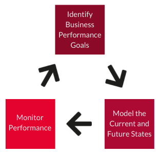
The method used to arrive at this customise approach and deliver a successful process factory performance improvement strategy consists of 3 ingredients:

Begin with the business goal in mind
Model the current and future states
Monitor performance

This method should be influenced by all the techniques, metrics and ways of working described in the previous sections.

The endgame here is to maximise the business benefits that accrue when undertaking improvement activities while minimising the waste of scarce human resources and minimising the under-utilisation of expensive capital assets.

Remembering that the scarcity of human resources and the exceptional cost of assets is what distinguishes the process industry from the car and assembly industry.

1 - Begin with the business goal in mind

Begin with the end in mind is a well-used phrase made popular by Stephen Covey in his book 7 habits of highly effective people.

Here we need to begin with the business goal in mind.

Said in other ways:

Understand intended actions in the light of anticipated consequences
Keep the main purpose in mind and think back from the final goal through whatever, sometimes complex, means and obstacles are required to achieve it.
Grasp current actions as part of a longer-term plan.

We believe there are 3 parts to defining robust business goals for a factory performance effort, shown below.

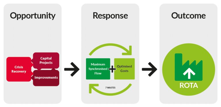
Opportunity

There are plenty of targets and this is always the case in the process industry. Combine this with the fact that there are less humans in the process industry to do the work then it is easy to see why opportunities must be prioritised.

There are always 3 types of opportunity within a factory as shown above: Crisis Recovery, Capital Projects, and Improvements. These opportunities are not made equally and they must be prioritised.

If products are about to be de-listed with your most important customer on a line that is out of capacity (Crisis) then it is pointless improving the shadow boards on another line that gets used 20% of the time (Improvement). Sorry …. it is just pointless!

If there is a major capital activity occurring at a process factory then resources that are normally committed to continuous improvement activities will probably need to be redirected towards nurturing a risky and complex capital project into their operating environment.

Continuous improvement activities can, and should, be put on hold in the pursuit of exceptional long term factory performance. This is a truism.

Response

The response to any opportunity (above) should support a virtuous circle in which synchronised flow is being maximised, costs optimised and waste minimised (see graphic below).

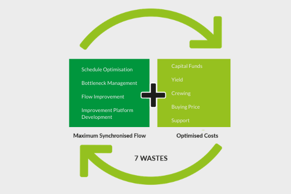
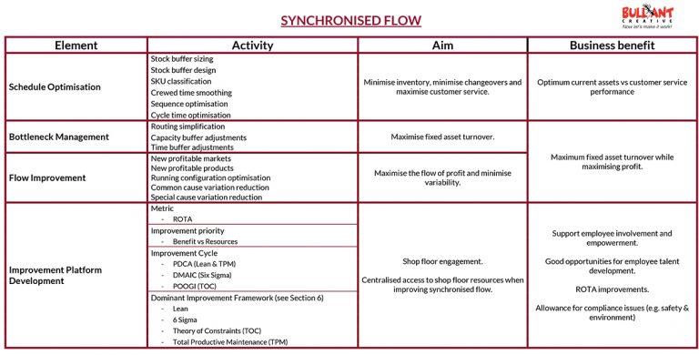
The table below shows more detail on Synchronised Flow in a process factory.

Notice that traditional continuous improvement frameworks form only part of a robust improvement platform from which broader business improvements can be added and sustained. This is something of a paradigm shift!

There have been many cases where the number of opportunities has increased because of a poor response to a previous opportunity.

For example, a buyer tries to minimise (not optimise) buying price by reducing the quality of raw material inputs (a distortion of what was originally a good opportunity) which causes a reduction in processing machine performance. This increases crewing costs, increases support resources (e.g. maintenance costs) and reduces yield (all together reducing synchronised flow). This increases the number of opportunities in the supply chain as well as causing a net reduction in business performance (reducing ROTA).

Selecting a good response to an opportunity within a complex processing factory is sophisticated. Done well it creates a virtuous circle that exceeds expectations. Selecting a poor response to an opportunity almost always causes a net reduction in business performance and leaves an insidious weakness in the operating system.

A ranking of a business opportunity should always be measured assuming the resources that will be needed to deliver the right response not the most expedient response.

Outcome

In the end, the success of a business is measured by Returned On Total Assets (ROTA).

When prioritising opportunities the final arbiter should be ROTA. The projected ROTA should be assessed while taking into consideration the most effective (not expedient) response.

I can hear the advocates for corporate responsibility (e.g. safety, environment, etc) crying foul here! Perhaps there is an additional measure apart from ROTA or you could just argue for a longer view of ROTA.

2 - Model the current and future states

So, the business goals for a factory improvement strategy have been decided after reviewing the opportunities at hand, understanding the most effective (not expedient) response for each opportunity and ensuring that the opportunities selected can deliver an improvement in ROTA.

The next step is to ensure that the opportunity can be broken into smaller, Performance Centred Improvements. Performance Centred Improvements are different to Continuous Improvements in that they deliver a large and measurable improvement in factory and business performance.

For this to be achieve with confidence, the opportunity must be capable of being modelled. The model must be presented in the current state and the future state. The difference between these 2 models is simply the benefits that can be accrued by the Performance Centred Improvements.

Here is a list of modelling techniques that can be applied within a complex process factory.

Financial Modelling (e.g. NPV)
Discrete Event Modelling
Constraints Modelling (Bullant Filters)
Spreadsheet Modelling
Value Stream Mapping

Check out this short video to see how we go about constraints modelling using the Bullant Filters.

3 - Monitor performance

This is probably the most important part of this ultimate guide to process factory performance and yet it is the bit that is almost always overlooked.

If you cannot or do not monitor factory performance against the current and future state models, then it makes modelling just an intellectual exercise.

Models must represent reality in order for them to add any value. If monitored behaviour of the factory cannot be linked to either the current state or the future state models then there is something wrong.

If the performance centred improvements are undertaken without the expected increase in monitored performance then there must be something wrong with the models or there must be something wrong with how the system is being monitored.

A modelling exercise that is undertaken without appropriate monitoring system is probably being used to define “stretching goals” or fulfil some sort of corporate reporting requirement. A modelling exercise used in this way is a modelling exercise which is doomed from the outset.

Finally, like all good adaptive and improvement systems there needs to be a feedback loop. Business priorities change so the modelling and monitoring activities should be adjusted accordingly.